Input Format
The input for Kfits is the raw results from kinetic measurements in a textual comma-separated or tab-delimited format, with the first column representing time and the second column representing some measure of protein aggregation or fibril formation. For example, the first column may contain time in seconds and the second may represent light scattering at 360 nm in arbitrary units.
The line preceding the first line of data is assumed to contain the text "XYDATA" and the data is followed by a blank line. A period of baseline measurement is expected to precede the actual aggregation process, and the aggregation is assumed to continue until the end of the measurement.
Flags and Parameters
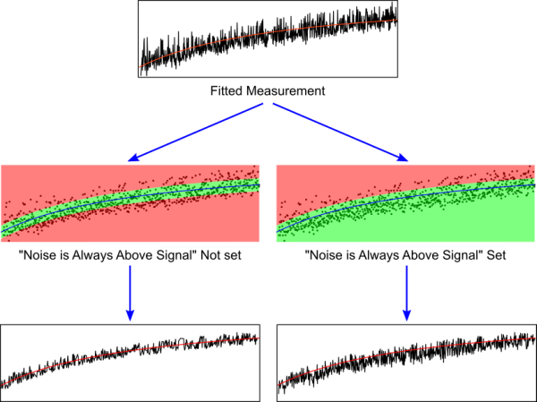
After fitting the measured data with the chosen model function, Kfits removes data points that are far from the theoretical curve ("TC"). The threshold (noise threshold, "NS") for the distance from the curve is estimated by the algorithm described above and can be overridden by the user. When the user choses not the set the "Noise is Always Above Signal" flag, every point residing outside of the TC ± NS band is marked for removal and removed; if the flag is set, only points with recorded values larger than TC + NS are removed. This flag is recommended for light scattering measurements, where air bubbles randomly cause excessive scattering.
Workflow
Step 1. Loading Data and Setting Parameters. The user choses a file and uploads it to the system, which plots the original measurement to the screen. The user can then choose the parameters for the fit. These include the kinetic model to be used (an automatic best-fit option is available) and the "Noise is Always Above Signal" flag, explained in the figure below. Finally, the setting "Process Reached Plateau During Measurement" determines whether the software should search for a period of plateau at the end of the measurement, after the end of the kinetics - or not; if in doubt, try both options and see which one produces a better fit.

Step 2. Setting the Margins of the Signal. In many cases, certain areas of the kinetic plot contain only noise, easily identifiable by the researcher. Two adjustable two-segment lines represent "only noise above this line" (green) and "only noise below this line" (red), allowing you to remove obvious noise.
Step 3. Setting Approximate Start of Kinetics Curve. Kinetic measurements often start with a baseline measurement, followed by addition of the components that create the observable signal. This setting has two effects: measurements before the chosen time point are used by the software to determine baseline values; and the model fit is assessed only according to data points after this point.
Step 4. Fitting a Function to the Data. The software will now try to fit the chosen model to the data using non-linear least-squares regression. It will then try to optimise the noise threshold, which can also be manually set by the user. Any datapoint residing outside the "signal band" will subsequently be removed.
Step 5. Downloading Clean Data and Reviewing Kinetic Parameters. At this final step, you can review your clean data as well as the calculated kinetic parameters. Then you can potentially adjust the noise threshold to achieve cleaner results or reduce loss of data, as well as download the clean results in textual format to your computer.
The Example Data
See "About" for details on the example data.
Further Instructions
Adding Support for Other Kinetic Models
The module kmodels.py describes the kinetic models that can be used by Kfits.
Each model is described by three constants: a function named FIT_<yourmodel>_INIT returning the default values for the parameters, a tuple named FIT_<yourmodel>_PARAM_NAMES containing the names of the parameter (allowing HTML tags) and the model itself represented by a parameterized function receiving time (t) as the first parameter and returning the expected y value at that time.
Parameter Initiation Function
This function receives two parameters: The apparent maximum value and the calculated baseline. Based on this very basic information the function should approximate
very grossly the parameters of the kinetic model, and return them in a tuple in the same order in which they will be constantly used in this model. These approximations will be used as the starting point from which the regression algorithm can begin fitting the model to the data.
For example, if we use the basic one-site binding model, i.e. y = (t * v
max) / (t + t
½):
def FIT_BASIC_INIT(apparent_max, baseline):
    approx_vmax = apparent_max - baseline
    approx_thalf = 12
    return (approx_vmax, approx_thalf)
Parameter Name Tuple
This is simply a tuple of names, which may contain html tags. These are used for displaying the fitted model parameters to the user at the end of the fitting process.
For example:
FIT_BASIC_PARAM_NAMES = ('v<sub>max</sub>', 't<sub>½</sub>')
The Model Function
This function is the most important part of the model definition, as it implements the integrated rate law that should be fitted to the data if this model is correct. The function simply receives t, i.e. the value on the x axis, as well as the values of all the kinetic parameters of the model by the same order used in the parameter initiation function. It returns the prediction of the y value at that time point for the given values of the kinetic parameters.
For example:
def fit_basic(t, vmax, thalf):
    return (t * vmax) / (t + thalf)
Registering the Model
After implementing the three components of a model, the model should be registered by adding it to the return value of the function get_models (in the same module). This function returns a dictionary, in which keys represent short simple names of models (which should not contain spaces or special characters) and values are four-tuples. The four-tuple for a model is comprised of the model function, the parameter initiation function, the parameter name tuple, and a long human-readable name for the model - in that order.
For example:
{'basic': (fit_basic, FIT_BASIC_INIT, FIT_BASIC_PARAM_NAMES, 'Basic One-Site Binding')}
Once the model is registered, the kfits server should be started (or restarted if it was running), and the new model will appear in the model choice box as well as being considered in the automatic model selection algorithm.
This software was intially written in September 2016 for Oded's personal use, and soon after extended to include a GUI for the comfort of the rest of the lab. By January 2017, the efforts to make it globally available, easy to use and as free as possible of bugs have begun. Finally, in May 2017, Kfits was ready to be sent out to the world.
The Example Data
Kfits comes with three example datasets, which were added to help the user play with the different settings of the software and understand their effects on the fit. Below are explanations about the sources of these example data and what they represent.
Example 1: Simulated Nucleation-Elongation
This
simulated example was built to be a perfect fit for the Nucleation-Elongation model. Noise was added primarily above the signal (random numbers between -5 and +35 were added to each datapoint), and thus
Kfits may perform better with the "Noise is Always Above Signal"
set. The aggregation kinetics continue until the end of the "measurement", or possibly even afterwards, thus no plateau period is observed and the data are best fitted with the "Process Reached Plateau During Measurement" flag
unset. Try changing the model to the one-site binding model or the automatic choice to get a feeling of how this system works.
Example 2: Simulated One-Site Binding
This
simulated example was built to be a perfect fit for the One-Site Binding model. Noise was added on both sides of the signal (random numbers between -35 and +35 were added to each datapoint) - "Noise is Always Above Signal" is better
unset. A plateau period with a slight decrease in signal (often seen in real measurements due to slow precipitation of aggregates) follows the kinetics and thus the use of "Process Reached Plateau During Measurement" is recommended.
Example 3: Real life Citrate synthase Aggregation Measured by Light Scattering
This is real data measured by Oded, showing the aggregation of chemically unfolded Citrate synthase upon dilution into a buffer containing a chaperone that decreases the rate and intensity of aggregation. For this example we recommend the One-Site Binding model, with "Noise is Always Above Signal"
set and "Process Reached Plateau During Measurement"
set. The fit is not perfect - but the important part is the
cleaning, for which the fit doesn't have to be perfect, only good enough; a noise threshold of 6 yeilds the best results in our opinion.
